TLDR; Notebook necessary to explore this machine-learning process hands-on and generate all the graphs below is available on my github

What is dropout and how can we use it to quantify uncertainty?

Dropout is a method of systematically inactivating certain elements of the layers of your neural network. Its primary use is implementing regularization and there are great tutorials like this one that outline that use case. Here however, we assume you’ve got a basic understanding of that implementation and we’re looking more toward how to hijack dropout for uncertainty quantification. In the previous posts we’ve talked about uncertainty quantification and why you might want to do it, but here we narrow down specifically on adversarial challenges and outlier detection

The MNIST dataset and defining our question(s)

A central task for ML algorithms is classification – you see learn to recognize a bunch of hand drawn numbers (like in the MNIST dataset) and you get pretty good at it. However what happens when I give a neural net trained on numbers is given a letter?

Well, it will give you an answer and that answer will be wrong. ML algorithms in general are built to answer specific questions - when they are given a challenge outside of that domain they tend to face plant. Here, we’re going to take a look out how we can leverage dropout to build a layer that rejects questions our algorithm is un-prepared to handle.

There are lots of ways to test this problem, but for us we’re going to train on the MNIST data-set (hand-written digits 0-9) and challenge with select letters from our EMNIST data-set (letters, see above). If our algorithm gives us correct responses for reject/accept on “is it a number?” and correct classifications on “what number is it?” it’s doing its job right.

Building a model that classifies handwritten digits and rejects adversarial challenges

First we need to build the super basic model. The MNIST dataset is quite easy to solve generically, so here we’re basically creating a placeholder model.

def basic_CNN():
    model = Sequential()
    model.add(Conv2D(32, (3, 3), activation='relu',
                                 input_shape=(28, 28, 1)))
    model.add(MaxPooling2D((2, 2)))
    model.add(Flatten())
    model.add(Dense(100, activation='relu',
                         kernel_initializer='he_uniform'))
    
    model.add(Dropout(0.25)) #<--- This bit is essential
    
    model.add(Dense(10, activation='softmax'))
    model.compile(optimizer='adam', loss='categorical_crossentropy', metrics=['accuracy'])
    return model

The next question is : how does this fit into our pipeline? We want to have a first pass that says “no, this is not a number!” before getting handed off to this classifier. The overall structure is going to look like this:

Rejecting adversaries relies on systematic differences in uncertainty between “known” and “unknown” samples

Lets start with a relative stripped down example. We trained the CNN described above with and without the dropout layer included. Now we’re going to do predictions on two sets of images : one set to test (the number 3) and one set to challenge (the letter N). We’re going to perform 10 predictions for each image and generate summary statistics using the code block below:

def compute_dropout_uncertainty(model,X,n_iter = 10):
    partial_model = Model(model.inputs, model.layers[-1].output)
    result = []
    for _ in range(n_iter):
        result.append(partial_model(X,training=True))

    result = np.array(result)

    prediction_mean = result.mean(axis=0)
    prediction_std = result.std(axis=0)
    return prediction_mean,prediction_std

The prediction_std term is the Uncertainty. Our hypothesis is that adversarial challenges will have above average uncertainty for our neural network. Plotting the values for both 3 and N shows this to be true, for the model that has dropout.

To put it in plain terms, if you don’t have dropout you can’t get any variance in this method. However if you do include dropout you can get pretty good separation between our 3 and N data

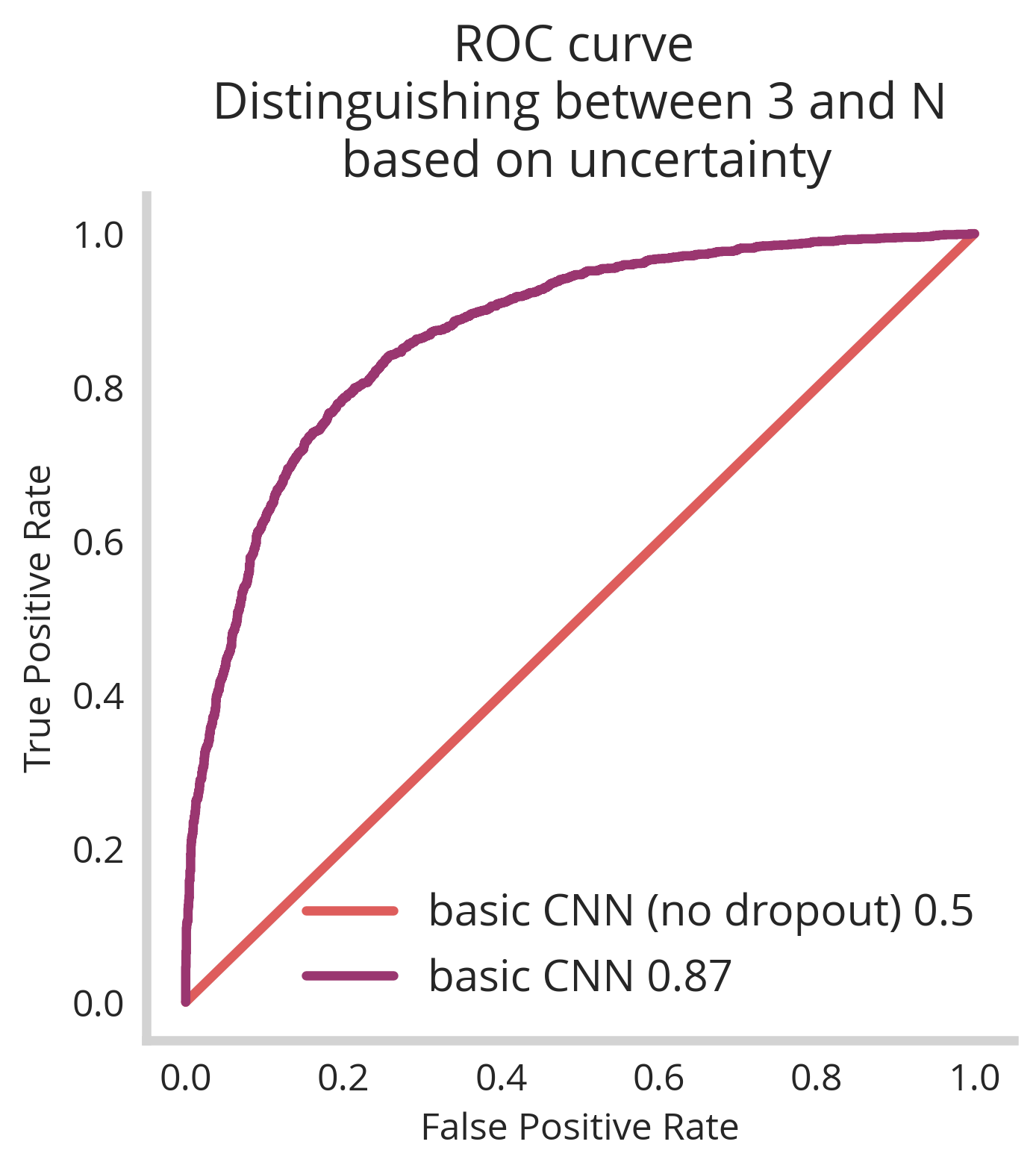
So we see that that based on the our dropout UQ we’re able to classify between “3” images as being within or wheelhouse and “N” as being adversarial. Simultaneous to this, we see that the basic CNN has a decent accuracy score of 0.9875.

However! We notice that when we apply it to all our adversarial examples, we only get an AUC of 0.81 – not super great. Lets see if we can identify why this is and train a slightly more sophisticated model to resolve it.

Deeper models perform better

By training our limited model on our MNIST dataset and testing on our adversarial EMNIST dataset, we see that there are uncertainty differences between letters and numbers. However, for this particular architecture these distributions are not completely distinguishable.

To solve this we will use a slightly expanded CNN architecture

def deep_CNN():
    model=Sequential()
    model.add(Conv2D(32, (3, 3), activation='relu', input_shape=(28, 28, 1)))
    model.add(BatchNormalization())
    model.add(Conv2D(32, kernel_size = 3, activation='relu'))
    model.add(BatchNormalization())
    model.add(Conv2D(32, kernel_size = 5, strides=2, padding='same', activation='relu'))
    model.add(BatchNormalization())
    model.add(Dropout(0.4))
    model.add(Conv2D(64, kernel_size = 3, activation='relu'))
    model.add(BatchNormalization())
    model.add(Conv2D(64, kernel_size = 3, activation='relu'))
    model.add(BatchNormalization())
    model.add(Conv2D(64, kernel_size = 5, strides=2, padding='same', activation='relu'))
    model.add(BatchNormalization())
    model.add(Dropout(0.4))
    model.add(Conv2D(128, kernel_size = 4, activation='relu'))
    model.add(BatchNormalization())
    model.add(Flatten())
    model.add(Dropout(0.4))
    model.add(Dense(10, activation='softmax'))
    model.compile(optimizer='adam', loss='categorical_crossentropy', metrics=['accuracy'])
    return model

This allows us to compare fully the two models basic and deep :

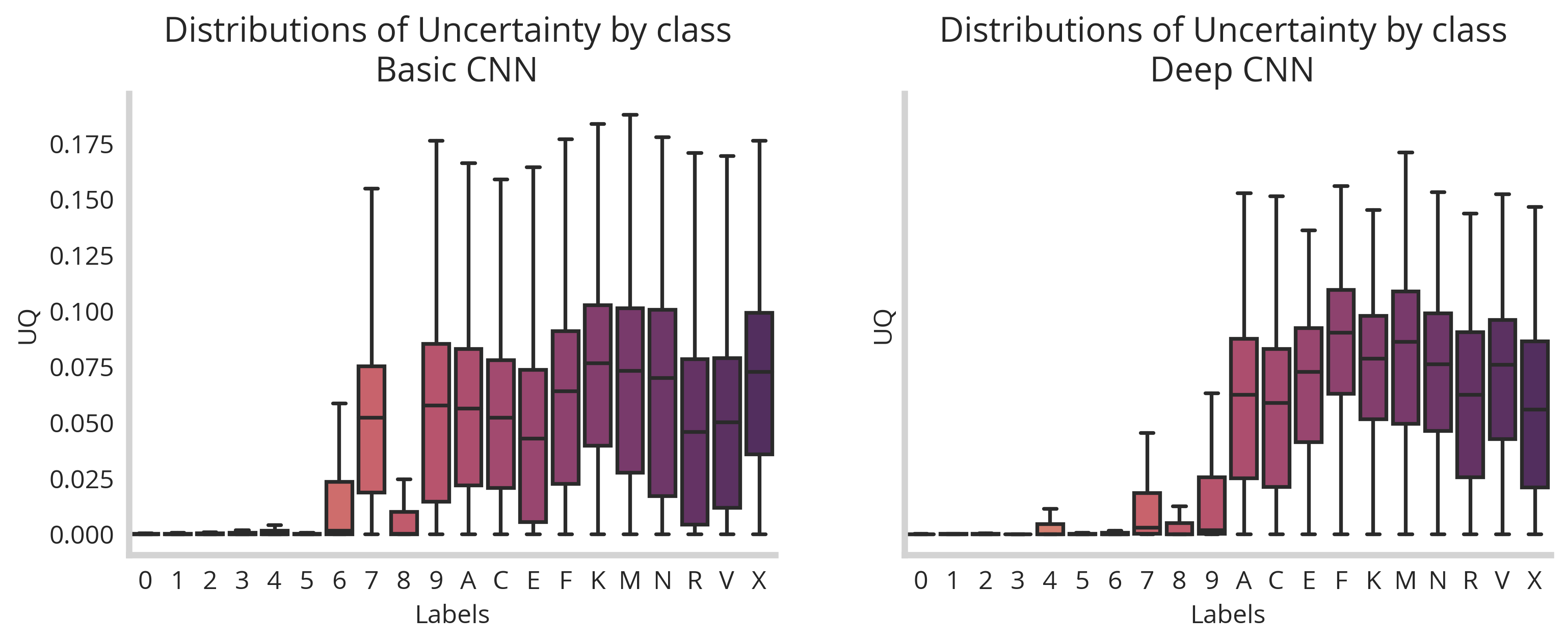
This difference in the class by class breakdown of generated uncertainty allows us to train a better logistic classifier for our deep_cnn data.

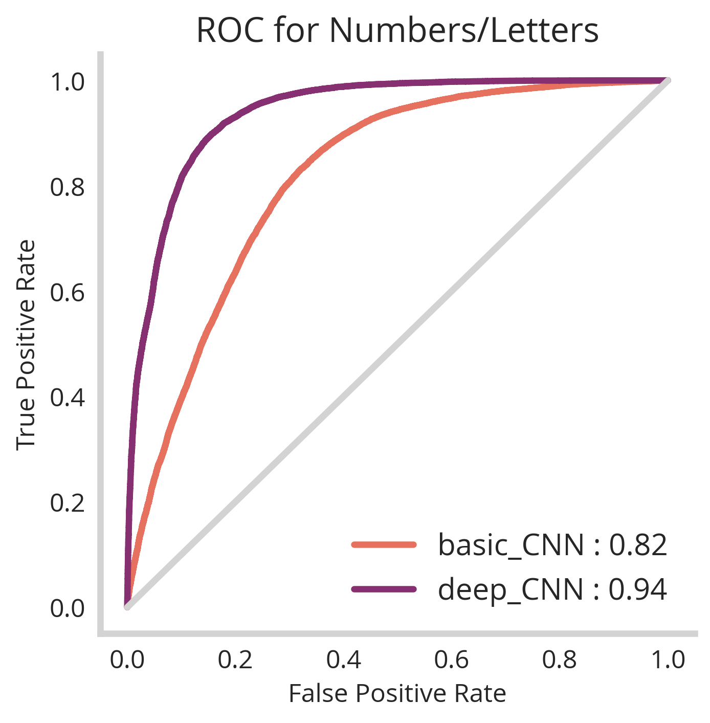
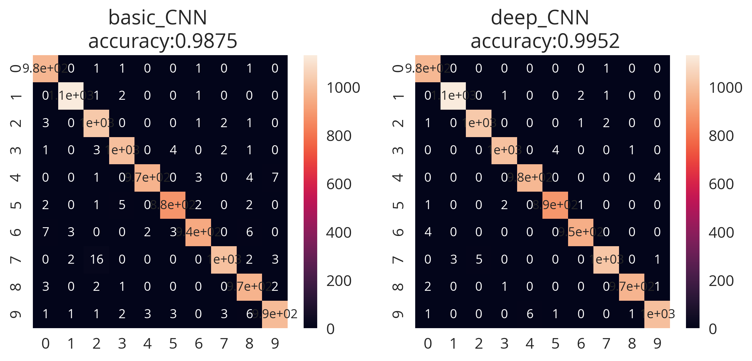
Still not perfect, but good enough for our toy example. We are seeing systematic differences between letters and numbers in terms of uncertainty. Overall for our deep_CNN, we have an accuracy score of 84% which could be tuned to reject or accept more depending on the tolerances of our production system. Of course, the MNIST classifier portion works well with >99% accuracy.

Ultimate test: challenging with hand-drawn, unfiltered images from my ipad

The ultimate test of our model is using things drawn by me, outside the context of training data. See the examples below:

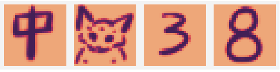
Here we have 4 exemplars: the chinese character 中, a poorly drawn baby yoda and two digits (3 and 8)

We load our previously trained model and make predictions on these new challengers:

resurection=DropoutMinstModel(base_model=deep_CNN,
                              n_epochs=30,
                              n_dropout_shuffles=100,
                             previous_trained_models='serialized_data/deep_cnn')
                             
                             
def rgb2gray(rgb):
    # this function gets hand drawn PNGs to look like MNIST charecters
    resultant=np.dot(rgb[...,:3], [0.2989, 0.5870, 0.1140])
    resultant = resultant.reshape((1, 28, 28, 1))
    return 1-resultant

img_loc='figures/yoda.png'
img = mpimg.imread(img_loc)     
yoda = rgb2gray(img)

img_loc='figures/zhong.png'
img = mpimg.imread(img_loc)     
zhong = rgb2gray(img)

img_loc='figures/3.png'
img = mpimg.imread(img_loc)     
hand_numb = rgb2gray(img)

img_loc='figures/8.png'
img = mpimg.imread(img_loc)     
hand_numb2 = rgb2gray(img)

all_test=np.vstack([zhong,yoda,hand_numb,hand_numb2])

resurection.predict(all_test)

How do these perform?

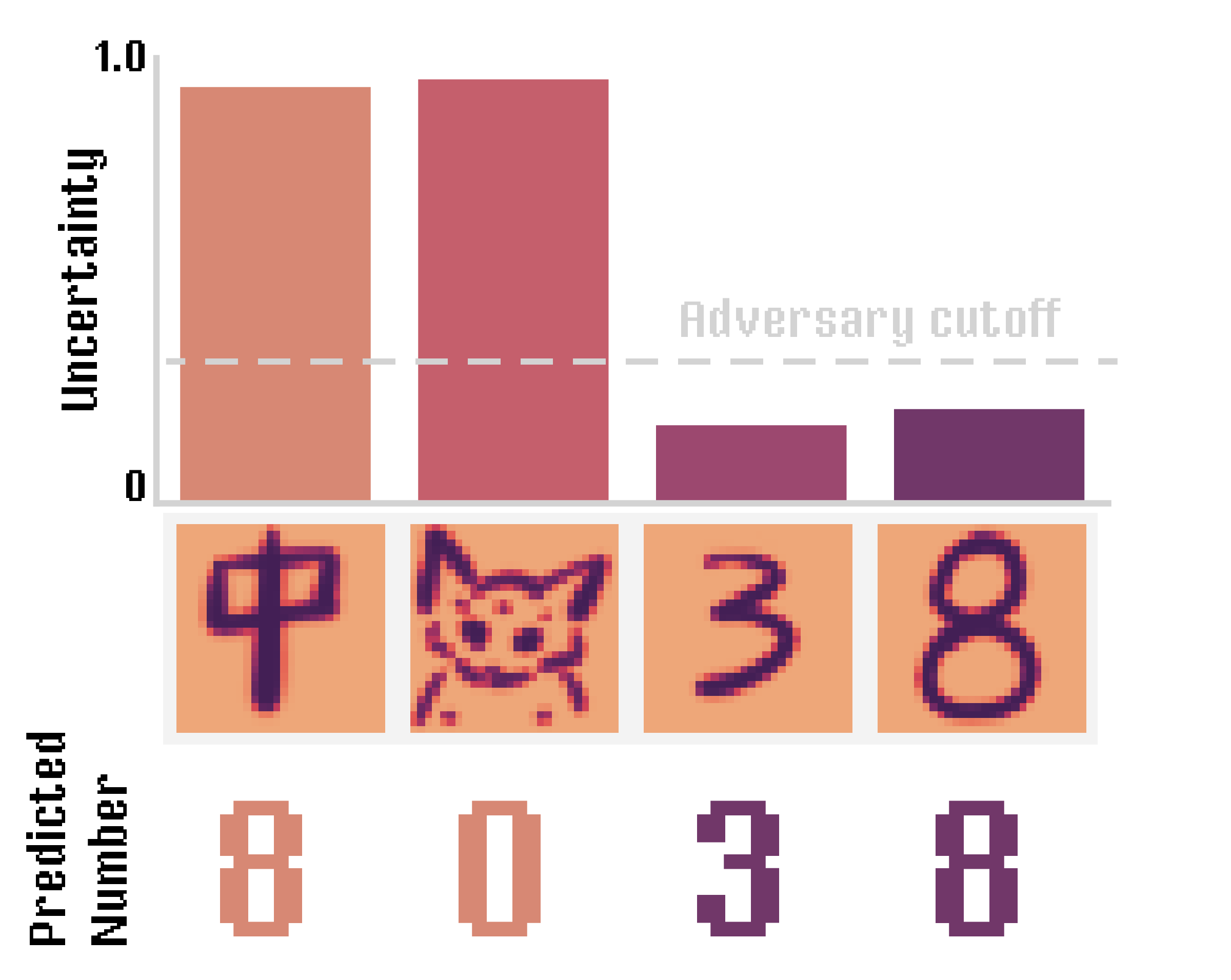
So looks like everything performs perfectly! Those that have higher uncertainty (中 and bbyoda) are classified as adversaries, numbers are classified as numbers and the correct number is assigned.

Epilogue : why not just use ensembles?

Previously we identified how to ensemble methods with sub-sampling of the data to get robust quantification of uncertainty. You can completely use this method here, but there are several advantages to each method:

Dropout-based UQ

• Can be performed on an existing model that was not built for UQ! No need for retraining! Simply load the model and use the dropout resampling snippet from above.
• Only requires the training of one model –> cuts down on computation time and model storage.
• For complex models, you need to do hundreds or thousands of interactions of dropout shuffling to correctly estimate uncertainty. This is intractable to train ensembles for.

Ensemble-based UQ

• Ensemble methods tend to give more robust predictions in general
• K-fold training of member models yields more accurate predictions than one model alone.
• Does not require that dropout be part of your layers (one less hyper-parameter to tune).

Notes

• Notebook necessary to generate all the graphs and more here
• The rest of the model and helper scripts here
• Previous posts on ensemble methods here
• Further reading from the paper that inspired this here